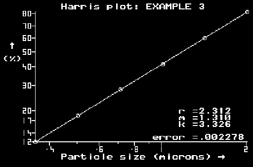
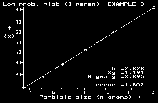
This is a computer program designed to plot distributions of particle size (or any other distributions or grade efficiency curves) into different coordinate systems in order to find one that yields a straight line and determine the parameters for the corresponding equation.

The method used is an analog of what particle size analysts have done manually for years: plotting data into different graph papers and, having found one in which the data fit a straight line, then reading the parameters for an equation from such a plot. Given the advantages of a computer, such plotting is done fast, without errors (once the numbers have been keyed in correctly) and a lot more information can be computed or otherwise extracted from the data than was possible or feasible manually.
The data are keyed in in the cumulative form, as percentages undersize versus particle size. A succession of plots then follows, either selected individually from a menu or in the following sequence (by pressing the space bar): linear plot, log-linear plot, log-log (Schuhmann) plot, Harris plot (3-parameter) (Schuhmann when r=1 or Gaudin-Meloy when m=1), Weibull plot (3-parameter) (Rosin-Rammler when a=0), Log-probability plot, Log-probability (3-parameter) with an upper bound. The functions are listed in the manual in the cumulative form (as fraction undersize).

Unless otherwise stated, most of the plots are based on 2-parameter functions commonly used in practice. A simple and elegant computational technique is used to find the best visual fit (minimum sum of squares in graphical coordinates), compute the two parameters for the representing equation and plot the best straight line through the data. The fit may be checked visually and, also, by asking for the value of minimum sum of squares corresponding to the line displayed. This value can then be compared with those from the other plots and the best - fitting function selected.
For the three-parameter equations, the third parameter is variable by hand (using an arrow key) so that its effect on one of the two axes and on the closeness of the fit can be observed. This is a highly educational feature which allows manual "optimization" of this third parameter (with the other two being found for each setting using the same method as for the two-parameter equations). There is a provision in the program to do this optimization automatically (starting from a manually-determined estimate if required), at the touch of a key.
Another feature allows to import the last fitted function into the linear plot and see how close the fit is in the linear coordinates. The two or three parameters used in obtaining this plot are printed with the graph on the screen. Finally, a table can be printed or displayed, of the original data and the computed values of the best-fitting function, to allow direct numerical assessment of the fit.
The program is ideal for:

It should be borne in mind that this is not meant to be yet another statistical package but an analog of a manual and visual fitting of data in graph papers. The fit obtained, therefore, (when using the "best fit" feature) is the best looking one, in graphical coordinates and not necessarily the best one in terms of the actual differences, in linear coordinates. The fit, therefore, accepts the weightings to such differences as produced by each graph paper in turn. This is in direct analogy with manual fitting of data with straight lines - we seek the best looking fit in a particular graph paper.
Related topics:
|
Copyright © 1997-2019 Fine Particle Software. All rights reserved. Send comments and corrections to lsvarovsky@aol.com. |